
Judging judges (round 2)
Published:
Before you read this, if you’re a Chicago resident, make sure you check out Injustice Watch’s Judicial Election Guide and fill out your sample ballot! Also, my full methodology can be found here and my code can be found here.
Background
Judicial elections, like many parts of Chicago city politics, are a wonderful tool for ensuring public accountability from powerful state actors in theory, and (mostly) an undemocratic mess in practice. In case that in-depth analysis was unsatisfying, I encourage you to check out this article for more info on the politics, past and present, of judicial races (and stick around, because Injustice Watch is the best in the business when it comes to judicial reporting in Cook County).
This post is focused on only one of the many flaws in this system: the warped incentives facing judges because of a public and press that is hyperfocused on violence caused by those “let off easy”. In simpler terms, I’m talking about the fact that as a Cook County judge you can lock up every defendant that appears before you for as long as possible and never face real retribution; but if you give the wrong defendant a second chance, you might lose your career for it. If you don’t believe me, have a look at Chicago Tribune articles that mention judges by name. This isn’t to minimize the violence done by people who’d stood in front of a judge before. But in a state that has the greatest number of years unjustly served by exonerated individuals, it’s worth noting the disconnect here. Chicago’s public and press (with obvious exceptions) have for decades been ruthless in punishing judges for the lives cut short by their kindness; they haven’t paid much attention to the lives destroyed by their cruelty.
In spring 2018, though, an opportunity arose to rectify that. Cook County State’s Attorney Kim Foxx released sentencing records going back well over a decade. In a city not known for transparency, the decision to release and continually update that data may be the greatest legacy she leaves behind. It can be found here.
Creating the ranking
The first half of my code is dedicated to creating a “severity metric”. This is done by aggregating the data by judges, calculating
- The percent of prison sentences above the median for a given felony class (i.e. is a class 1 felony prison sentence above the median prison sentence given to a class 1 felony, etc…).
- The percent of class 4 felony sentences resulting in prison time.
I average those two measures to create my severity metric. I drop all judges who have served on less than 500 case (I like to deal in large sample sizes; the outcomes for judges who haven’t served on many cases could be misleading). From there I abbreviate the list and order it to make it tidy. I export the full list of 90 judges, ranked, to a CSV you can find here. Below you can see the judges included in the list who are on the ballot for retention November 3rd, with their relative rank within the list of 90 judges by my severity metric.
| Judges | % prison/jail sentences above median | % Class 4 felonies sentenced to prison/jail | Severity metric | |
| 3 | URSULA WALOWSKI | 0.505 | 0.670 | 0.588 |
| 24 | Araujo, Mauricio | 0.522 | 0.559 | 0.540 |
| 25 | Byrne, Thomas | 0.537 | 0.538 | 0.538 |
| 28 | William Raines | 0.347 | 0.712 | 0.529 |
| 38 | Kenneth J Wadas | 0.458 | 0.572 | 0.515 |
| 55 | Anna Helen Demacopoulos | 0.489 | 0.481 | 0.485 |
| 64 | Shelley Sutker-Dermer | 0.411 | 0.502 | 0.456 |
| 70 | Kerry M Kennedy | 0.352 | 0.534 | 0.443 |
| 75 | Steven G Watkins | 0.367 | 0.496 | 0.431 |
Checking significance
A ranking is one thing, but for context we want to see if the judges at the top of our ranking do seem to hand down “severe” sentences at a significant rate. Otherwise, the differences we see in the variables that make up our severity metric (percent of prison sentences “above the median” and percent of class 4 felony sentences resulting in prison time) could just be statistical noise.
Two years ago, when I was only looking at Judge Maura Slattery Boyle, I did this by “bootstrapping”, i.e. resampling data with replacement. My logic was that doing it this way I wouldn’t have to assume the distribution of the statistic (in this case, the two aforementioned variables). I could draw a 95% confidence interval around the variables for Judge Slattery Boyle, and then compare that confidence interval to the actual values of the variables in the entire population. If the bottom end of the confidence interval was above the actual value of the variable in the entire dataset (which was the case), I could say at a p-val of .05 that Judge Slattery-Boyle’s sentences weren’t randomly picked from the population at large. In other words, she was sentencing at a higher rate than the “average” judge.
In retrospect, this approach wasn’t particularly elegant or effective. I didn’t want to do a simple linear regression because I was dealing with two dummy variables, and the distribution of the regression residuals wasn’t even close to normal. My understanding then (and now, although I’d love if someone could walk me through this like I was 5) was that while non-normal residuals don’t violate the Gauss-Markov theorem, they did make it impossible to interpret the t statistics/p-values produced, and the p-value was all I really wanted.
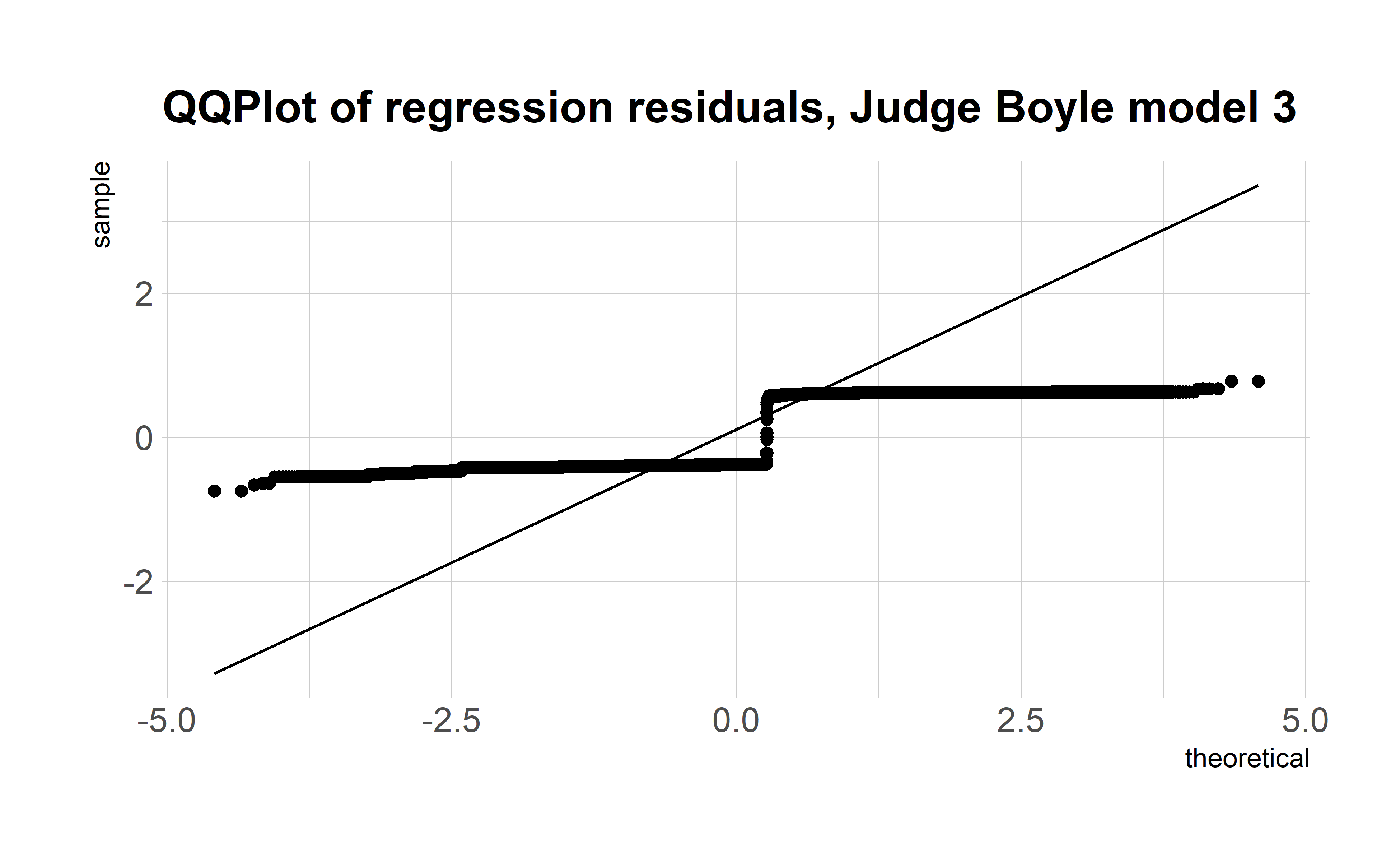 Look at how ugly these residuals are
Looking back now, I’ve had a change of heart for three reasons.
- As long as the Gauss-Markov assumptions are satisfied (we can adjust for heteroskedasticity using robust standard errors), the coefficient produced by my linear regression is still BLUE and consistent, meaning that given the massive sample size offered by this data (well over 100k cases), I feel more comfortable interpreting the coefficient than I did then.
- The biggest concern I always had was omitted variable bias, and by using a linear regression to assess significance I’m able to control for two additional variables that I didn’t account for in my bootstrap method: sentence date (as a continuos variable, assuming sentences have gotten more lenient over time) and sentence years (as fixed effects, assuming sentencing norms/rules might change year to year).
- I can test my assumption in (1), that my OLS coefficients are trustworthy because the sample size is so large, by A) running logistic regressions of the same models, since logistic regression p-vals don’t presume normality of residuals, and B) using bootstrapping to construct a distribution of my coefficient of interest (across bootstrapped samples of my data), and using that distribution to create an empirical confidence interval around my estimate.
At the bottom of this post I have five OLS and five logit regression tables for five judges: Maura Slattery Boyle (still leading by my severity metric, and I want to see if controlling for the additional covariates changes the results for her), Ursula Walowski, Mauricio Araujo, Thomas Byrne, and William Raines (all up for retention and in the top third of judges by sentencing severity). Each table has three columns for three dependent variables
- Dummy variable for sentence being above the median (0 if not, 1 if so, only using sentences that resulted in prison or jail time)
- Dummy variable for sentence being a class 4 felony and resulting in prison time (0 if class 4 felony sentenced to probation, 1 if class 4 felony sentenced to prison or jail, only using sentences on class 4 felonies where the outcome was prison, jail or probation)
- Dummy variable for a sentence being “severe” (1 if sentence is for prison or jail and “above the median” for that particular felony class OR if a sentence is for prison or jail and the charge is a class 4 felony, 0 otherwise, using all sentences on Class X-4 felonies resulting in prison, jail, or probation)
My model for each table is as follows: y_i = βdummy_i + αsentence_date_i +Xsentence_year_fixed_i, where “y” is our dependent variable, “dummy” is our binary variable for the case being heard by the given judge, “sentence_date” is the date the case was sentenced, and “sentence_year_fixed” is a matrix of dummy variables for the sentence years in our data (absorbing the fixed effects of each year). We regress across cases (i). Our variable of interest is β in each model.
The OLS coefficients for our judge dummy variables can be interpreted as increases in severe sentence probability (since our dependent variable is binary, our OLS model is a Linear Probability Model). So, for instance, the .103 coefficient in column three of Judge Slattery Boyle’s regression table means our model estimates a 10.3% increase in the likelihood of a severe sentence if a case is heard by Judge Slattery Boyle. It’s important to note that this increase is in comparison to the “average” judge. If your case was heard by Judge Raines, who also ranks high on severity metric, instead of Judge Slattery Boyle, your chances of a severe sentence wouldn’t decrease by 10.3% (or at all for that matter).
While t-statistics and p-values are included, they shouldn’t be considered in the OLS tables since they presume normality of residuals (they should be accurate in the logit tables though). The OLS coefficients themselves should be considered reasonably accurate estimates given the sample size (I’m inclined to trust their sign except for the ones extremely close to 0, i.e. abs(coef)<.05). As a sanity test for this presumption, I’ve also included a bootstrapped distribution of one of my models: the third column of Judge Slattery Boyle’s regression table (I’m not doing all the models because bootstrapping is a time and computing heavy task, and I’ve put my laptop through enough). Below you can see the summary of my bootstrapped coefficient, and a histogram/QQ Plot of its distribution. My 99% confidence interval (drawn around the percentiles of the distribution) is (.0803, .1290). If you compare these results with column three of Judge Slattery Boyle’s regression table at the bottom of this post, you’ll see that happily results line up pretty well (our regular OLS coefficient estimate is .104). Furthermore, if you consider the coefficients and p-values of the logit tables, they line up pretty much perfectly with the OLS tables.
I take the bootstrapping and logit results lining up with my OLS coefficients as a pretty good sign that the sample size is mitigating the impacts of our wonky residuals, and therefore our coefficients by and large are pretty robust. I welcome any critiques though. For the record, I’m not paying much attention to the logit coefficients beyond confirmation of my OLS model since the interpretation of logit coefficients is less natural than that of OLS coefficients.
| R | original | bootBias | bootSE | bootMed | |
| 1 | 5,000 | 0.104 | 0.0002 | 0.009 | 0.104 |
Bootstrapped regression output summary (coefficient is pretty much unchanged)
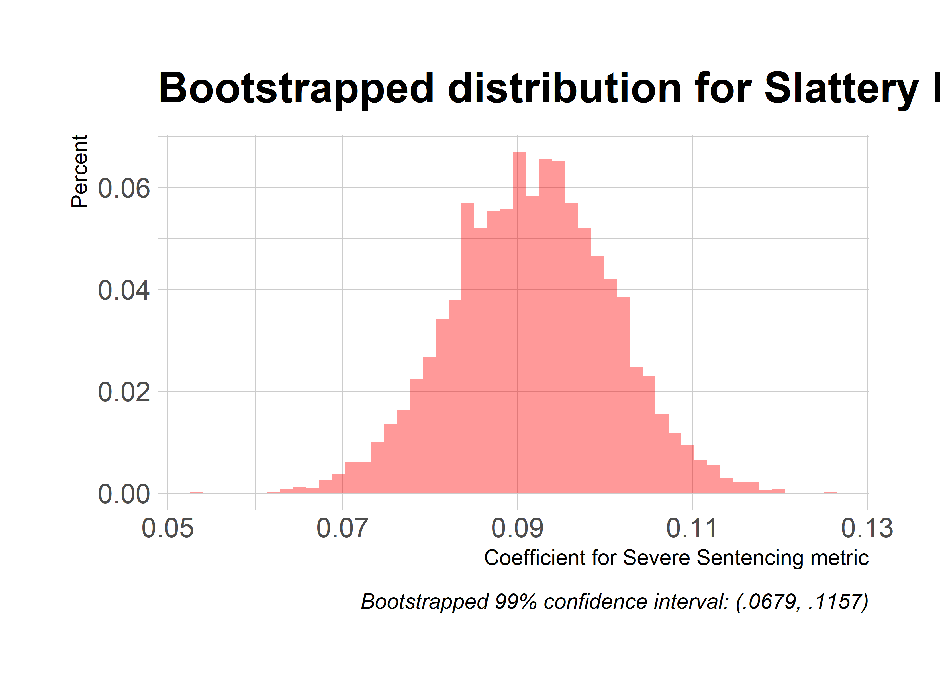 graphs of our coefficient distribution from the bootstrapped samples, showing a pretty neat bell curve around our estimated value
Conclusion/Next Steps
There’s a ton of work left to do here, and I hope my code serves as a jumping off point for others. Personally, I think the next step is developing a more rigorous index of “severe sentencing” than the binary I use now. The advantage of my current approach is
- It isn’t skewed by any one sentence, i.e. some absurdly long prison sentence for a class 4 felony, and therefore our findings are more concerned with consistent habits. I actually think this is a real benefit; some absurdly long sentence could be due to omitted variables, in which case it would distort our outcomes, and generally I’m more interested in judges that are consistently giving “severer than normal” sentences.
- It keeps me from making too many decisions in my index construction, which, given that I don’t have a law degree, I like. I’ve been scouring google scholar for two years now hoping to find some paper that goes into detail about what makes a sentence “severe”, but so far, no luck. Please send such work my way.
Approaching this from a linear regression standpoint has also given me newfound appreciation for my original approach, which was just to look at a sample with a seemingly high value of severe sentences (i.e. Judge Slattery Boyle’s cases) and calculate a p-value representing the likelihood that that sample occurred randomly. While the regression model lets me control for additional covariates, I can replicate that control without using a linear model and dealing with all the headaches of its p-value construction. Sometime in the next few months I think I’ll return to this data, and just break out a bunch of subgroups by strata I think are important (i.e. case year, felony class, general sentence charge). I’ll look at whether the judges my ranking suggests are especially harsh pass severe sentences more than the population at large in each of these strata, and then run a Fisher’s exact test to construct a p-value representing the likelihood there is a relationship between my two categorical variables. Again, all I really care about is whether the difference I see in severe sentencing percentages between a given judge and the “average” judge (i.e. the population generally) is statistically significant.
The greatest improvement in this analysis though would be the inclusion of criminal history as a control. Cases are assigned randomly, so in judges who have served on a lot of cases I’m not too worried about data being unfairly skewed (again, that’s why I restrict my ranking to >500 cases). It would still be really nice to have that information. Unfortunately, the Cook County courts have been unwilling to provide that data so far. I really hope that changes.
All in all, I see this as the fairest attempt I can make (right now) at measuring sentence severity and assessing its significance rigorously. I’d love to be proved wrong.
Sources Consulted
- For addressing non-normality of residuals: Frontiers in Psychology Review of approaches
- For bootstrapping regressions in R: Stanford Guide
- For OLS vs. Logit models when facing binary dependent variables: StatModeling Columbia blog post
Thanks to Ben, Owen, Peter and Professor Jayachandran for their advice on handling my p-val concerns.
OLS Regression Tables
Judge Slattery Boyle
| Dependent variable: | |||
| Above median sentence | Class 4 prison sentence | Severe sentence | |
| (1) | (2) | (3) | |
| boyle_dummy | 0.078*** | 0.132*** | 0.104*** |
| (0.011) | (0.013) | (0.009) | |
| sentence_date | 0.00002 | -0.00001 | 0.00000 |
| (0.00001) | (0.00002) | (0.00001) | |
| Constant | 1.246*** | 0.013 | 1.048*** |
| (0.193) | (0.018) | (0.147) | |
| Observations | 129,586 | 96,051 | 214,571 |
| Adjusted R2 | 0.002 | 0.004 | 0.001 |
| Note: | *p<0.1; **p<0.05; ***p<0.01 | ||
| Also controlling for sentence year fixed effects | |||
| Huber-White robust standard errors | |||
Judge Walowski
| Dependent variable: | |||
| Above median sentence | Class 4 prison sentence | Severe sentence | |
| (1) | (2) | (3) | |
| walowski_dummy | 0.042** | 0.125*** | 0.073*** |
| (0.017) | (0.021) | (0.015) | |
| sentence_date | 0.00002 | -0.00001 | 0.00000 |
| (0.00001) | (0.00002) | (0.00001) | |
| Constant | 1.231*** | 0.015 | 1.029*** |
| (0.193) | (0.018) | (0.147) | |
| Observations | 129,586 | 96,051 | 214,571 |
| Adjusted R2 | 0.002 | 0.004 | 0.001 |
| Note: | *p<0.1; **p<0.05; ***p<0.01 | ||
| Also controlling for sentence year fixed effects | |||
| Huber-White robust standard errors | |||
Judge Araujo
| Dependent variable: | |||
| Above median sentence | Class 4 prison sentence | Severe sentence | |
| (1) | (2) | (3) | |
| araujo_dummy | 0.052*** | 0.003 | -0.027** |
| (0.016) | (0.016) | (0.011) | |
| sentence_date | 0.00002 | -0.00001 | 0.00000 |
| (0.00001) | (0.00002) | (0.00001) | |
| Constant | 1.231*** | 0.015 | 1.034*** |
| (0.193) | (0.018) | (0.147) | |
| Observations | 129,586 | 96,051 | 214,571 |
| Adjusted R2 | 0.002 | 0.003 | 0.001 |
| Note: | *p<0.1; **p<0.05; ***p<0.01 | ||
| Also controlling for sentence year fixed effects | |||
| Huber-White robust standard errors | |||
Judge Byrne
| Dependent variable: | |||
| Above median sentence | Class 4 prison sentence | Severe sentence | |
| (1) | (2) | (3) | |
| byrne_dummy | 0.074*** | -0.015 | 0.023** |
| (0.015) | (0.018) | (0.012) | |
| sentence_date | 0.00002 | -0.00001 | 0.00000 |
| (0.00001) | (0.00002) | (0.00001) | |
| Constant | 1.234*** | 0.015 | 1.032*** |
| (0.193) | (0.018) | (0.147) | |
| Observations | 129,586 | 96,051 | 214,571 |
| Adjusted R2 | 0.002 | 0.003 | 0.001 |
| Note: | *p<0.1; **p<0.05; ***p<0.01 | ||
| Also controlling for sentence year fixed effects | |||
| Huber-White robust standard errors | |||
Judge Raines
| Dependent variable: | |||
| Above median sentence | Class 4 prison sentence | Severe sentence | |
| (1) | (2) | (3) | |
| raines_dummy | -0.124*** | 0.161*** | 0.115*** |
| (0.015) | (0.018) | (0.014) | |
| sentence_date | 0.00002 | -0.00002 | 0.00000 |
| (0.00001) | (0.00002) | (0.00001) | |
| Constant | 1.267*** | 0.018 | 1.011*** |
| (0.193) | (0.018) | (0.147) | |
| Observations | 129,586 | 96,051 | 214,571 |
| Adjusted R2 | 0.002 | 0.004 | 0.001 |
| Note: | *p<0.1; **p<0.05; ***p<0.01 | ||
| Also controlling for sentence year fixed effects | |||
| Huber-White robust standard errors | |||
Logit Regression Tables
Judge Slattery Boyle
| Dependent variable: | |||
| Above median sentence | Class 4 prison sentence | Severe sentence | |
| (1) | (2) | (3) | |
| boyle_dummy | 0.078*** | 0.132*** | 0.104*** |
| (0.011) | (0.014) | (0.009) | |
| sentence_date | 0.00002 | -0.00001 | 0.00000 |
| (0.00001) | (0.00002) | (0.00001) | |
| Constant | 1.246** | 0.013 | 1.048** |
| (0.535) | (0.498) | (0.513) | |
| Observations | 129,586 | 96,051 | 214,571 |
| Log Likelihood | -93,754.010 | -69,284.640 | -151,892.400 |
| Akaike Inf. Crit. | 187,584.000 | 138,625.300 | 303,876.700 |
| Note: | *p<0.1; **p<0.05; ***p<0.01 | ||
| Also controlling for sentence year fixed effects | |||
| Huber-White robust standard errors | |||
Judge Walowski
| Dependent variable: | |||
| Above median sentence | Class 4 prison sentence | Severe sentence | |
| (1) | (2) | (3) | |
| walowski_dummy | 0.042** | 0.125*** | 0.073*** |
| (0.018) | (0.022) | (0.014) | |
| sentence_date | 0.00002 | -0.00001 | 0.00000 |
| (0.00001) | (0.00002) | (0.00001) | |
| Constant | 1.231** | 0.015 | 1.029** |
| (0.535) | (0.498) | (0.513) | |
| Observations | 129,586 | 96,051 | 214,571 |
| Log Likelihood | -93,777.100 | -69,315.120 | -151,947.300 |
| Akaike Inf. Crit. | 187,630.200 | 138,686.200 | 303,986.600 |
| Note: | *p<0.1; **p<0.05; ***p<0.01 | ||
| Also controlling for sentence year fixed effects | |||
| Huber-White robust standard errors | |||
Judge Araujo
| Dependent variable: | |||
| Above median sentence | Class 4 prison sentence | Severe sentence | |
| (1) | (2) | (3) | |
| araujo_dummy | 0.052*** | 0.003 | -0.027** |
| (0.015) | (0.017) | (0.011) | |
| sentence_date | 0.00002 | -0.00001 | 0.00000 |
| (0.00001) | (0.00002) | (0.00001) | |
| Constant | 1.231** | 0.015 | 1.034** |
| (0.535) | (0.498) | (0.513) | |
| Observations | 129,586 | 96,051 | 214,571 |
| Log Likelihood | -93,774.380 | -69,331.770 | -151,957.300 |
| Akaike Inf. Crit. | 187,624.700 | 138,719.500 | 304,006.600 |
| Note: | *p<0.1; **p<0.05; ***p<0.01 | ||
| Also controlling for sentence year fixed effects | |||
| Huber-White robust standard errors | |||
Judge Byrne
| Dependent variable: | |||
| Above median sentence | Class 4 prison sentence | Severe sentence | |
| (1) | (2) | (3) | |
| byrne_dummy | 0.074*** | -0.015 | 0.023** |
| (0.015) | (0.018) | (0.012) | |
| sentence_date | 0.00002 | -0.00001 | 0.00000 |
| (0.00001) | (0.00002) | (0.00001) | |
| Constant | 1.234** | 0.015 | 1.032** |
| (0.535) | (0.498) | (0.513) | |
| Observations | 129,586 | 96,051 | 214,571 |
| Log Likelihood | -93,767.000 | -69,331.430 | -151,958.000 |
| Akaike Inf. Crit. | 187,610.000 | 138,718.900 | 304,008.100 |
| Note: | *p<0.1; **p<0.05; ***p<0.01 | ||
| Also controlling for sentence year fixed effects | |||
| Huber-White robust standard errors | |||
Judge Raines
| Dependent variable: | |||
| Above median sentence | Class 4 prison sentence | Severe sentence | |
| (1) | (2) | (3) | |
| raines_dummy | -0.124*** | 0.161*** | 0.115*** |
| (0.016) | (0.019) | (0.014) | |
| sentence_date | 0.00002 | -0.00002 | 0.00000 |
| (0.00001) | (0.00002) | (0.00001) | |
| Constant | 1.267** | 0.018 | 1.011** |
| (0.535) | (0.498) | (0.513) | |
| Observations | 129,586 | 96,051 | 214,571 |
| Log Likelihood | -93,750.210 | -69,297.430 | -151,925.100 |
| Akaike Inf. Crit. | 187,576.400 | 138,650.900 | 303,942.300 |
| Note: | *p<0.1; **p<0.05; ***p<0.01 | ||
| Also controlling for sentence year fixed effects | |||
| Huber-White robust standard errors | |||